Spatial Hydrology of the Urubamba River System in Peru

Spatial Hydrology of the Urubamba River System in Peru
Using Geographic Information Systems (GIS)

by Francisco Olivera, Ph.D.
Center for Research in Water Resources
University of Texas at Austin
January 1996

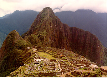
Figure 1: Macchu Picchu, one of the wonders of the Inca civilization,
is located few kilometers away from the Urubamba River.
(Photo by F. Olivera, 1989)

1. Introduction
2. Overview of the study site
3. Stream and Watershed Delineation
4. Using the Hydrologic Modeling Extension

1. Introduction

The purpose of this page is to give the reader a feeling of the potentiality of available-for-whole-world data, such as the 30 arc-second digital elevation model (DEM) and the Digital Chart of the World, when used in combination with the PC version of ArcView 3.0 and its extension Spatial Analyst. 30 arc-second DEM's (approximately 1 Km² square cells) for the entire world have been developed by the Earth Resources Observation Systems (EROS) Data Center of the United States Geological Survey (USGS), and can be downloaded from their internet site. Instructions for downloading, unzipping, and setting these DEM grids are available at How to Download a 30" DEM?. The Digital Chart of the World is a database of geographic features of the world, developed by the Environmental System Research Institute (ESRI).

The study site is the Urubamba River system located at the South-West of Peru in South America. Any region of the world could have been studied, and the case of the Urubamba river has been chosen more because of personal than of technical reasons. My familiarity with the region, undoubtedly, biased the selection of the study site, but that does not imply that knowledge of the area is required for identifying the basic spatial hydrologic features of the region.

This web-page does not attempt to be a complete analysis of the hydrology of the Urubamba River system, nor does it attempt to be an ArcView tutorial. It is just a demonstration of how far one can get using basic and available data handled with ArcView 3.0 in a personal computer (IBM or compatible).

Before you start

Download the following files located at the directory /export/home2/ftp/pub/gisclass/urubamba of danube.crwr.utexas.edu:

cities.dbf, .shp, .shx
cntry94.dbf, .sbn, .sbx, .shp, .shx
pe30dem.asc
roads.dbf, .shp, .shx
topo_shd.avl
ur_burn0.dbf, .shp, .shx

To import the ASCII file pe30dem.asc into a grid, star ArcView 3.0, go to File/Import Grids..., select ASCII under Select import file type and name it pe30dem.

If you are using the ur_burn0 shapefile, you may skip the first two steps of "Part I: Setting the DEM".

2. Overview of the Study Site

Peru is located at the north and a half of South America's West coast. It extends from latitude 0° to 19°S, longitude 68°W to 82°W, and has an area of 1'285,215.6 Km² (496,251.7 sq-mi). A view of the world seen from above Peru is shown in Figure 2.

Figure 2: The globe seen from above Peru.

The coverage presented in Figure 2, called cntry94.shp, was obtained from ESRI Data & Maps supplied with the ArcView 3.0 code. The original coverage is in Geographic Projection and has been projected into Orthographic Projection with central meridian 75°W and reference parallel 10°S.

To create a View of the world, click the View icon in the Project window, press the New buttom, go to View/Add Theme, select Feature Data Source under Data Source Types, and select the shapefile cntry94.shp. To change the name of the View, go to View/Properties and enter World in the Name slot. To display the View in Orthographic Projection, go to View/Properties, press the Projection buttom, check the Custom option, under Category select Orthographic, and enter the values of the Central Meridian and Reference Parallel mentioned above in decimal degrees.

Peru is crossed from North to South by the Andes, being its highest mountain, the Huascaran, 6,768 m (22,205 ft) high. Three water systems are found in the peruvian territory:

To the West of the Andes, dry and dessertic areas extend all the way to the ocean, being interrupted by fertil valleys formed by rivers that run East-West from the highlands.
To the East of the Andes, highly humid and almost flat areas, well known as the tropical rain forest, extend as part of the Amazon basin.
Within the southern part of the peruvian Andes, a high mesa called Collao extends around the border between Peru and Bolivia, and drains towards the Titicaca lake.

In a nutshell, all the land to the West of the Andes drains to the Pacific Ocean, that to the East of the Andes drains to the Amazon river, and that of the southern part of the peruvian Andes to the Titicaca lake. The Urubamba is part of the second water system, and (together with the Apurimac River) is the upper most tributary of the Amazon.

Create a View named Peru, and add the Themes dem30pe (grid data source), and border.shp, roads.shp and cities.shp (feature data sources).

A topographic map (i.e., a ramp-shaded presentation of the DEM) of Peru is presented in Figure 3.

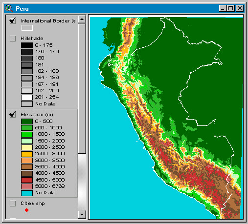
Figure 3: Topographic map of Peru, according to the USGS 30" DEM.

To display the topographic map of Peru with the color legend shown in Figure 3, click the theme bar in the legend area of the View to make dem30pe active (the theme bar will raise), go to Theme/Edit Legend, press the Load buttom, and select the file topo_shd.avl. The reader familiar with the area might be able to recognized the three water systems mentioned above.

A hill shade - 3-D like - representation of the peruvian territory is shown in Figure 4.

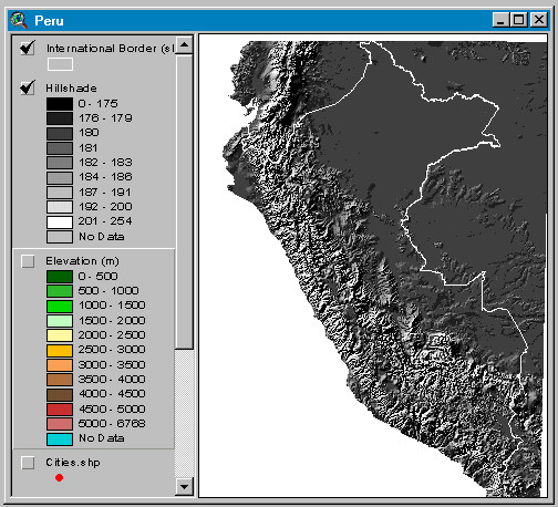
Figure 4: "Hillshade" map of Peru, according to the USGS 30" DEM.

To display the map of Peru as it looks in Figure 4, make dem30pe active, go to Analysis/Compute Hillshade... , and enter the parameters or accept the default ones.

The main cities and roads of Peru, according to the DCW, are shown in Figure 5.

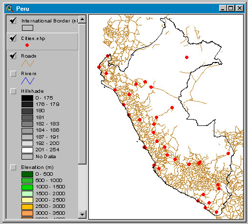
Figure 5: Cities and roads of Peru, according to the DCW.

Only 35 cities, out of the 2230 populated points included in the DCW, have been selected. These cities include the capitals of the former departamentos (equivalent to provinces or states), the main ports, the cities with important economic activity and Pisac (of course!).

The Urubamba River system is located in the southern part of Peru. A rectangular box of 410 Km (East -West) by 543 Km (North - South), that comprises the entire watershed, was selected for analysis purposes. A location map of this box is presented in Figure 6.

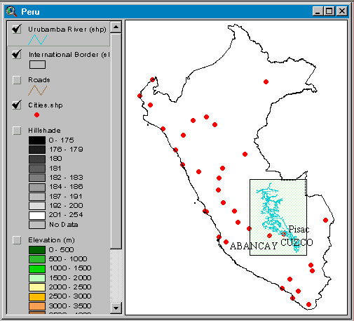
Figure 6: Location map of the study area. The map also shows the
Urubamba River system as well the main cities of the country.
Cities within the study area are labeled with their names.

Create a View named Urubamba, and add the Themes dem30pe (grid data source) and ur_burn0.shp (feature data source). To define your analysis extent, zoom-in to the Urubamba River watershed (the extent of Figure 7 can be used as a reference) making sure that the Northern reach of ur_burn0.shp flows out of the window and that the entire drainage area fits within the window, go to Analysis/Properties, and select Same as Dislay in the Analysis Extent slot.

The rivers of the area, according to the DCW, are presented in Figure 7. To make things clearer, the Urubamba river, as well as its main tributaries, have been colored darker.

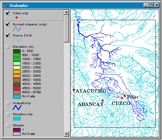
Figure 7: The Urubamba River and main tributaries (in dark blue),
and rivers of the study area (in light blue).

The topography of the area is presented in Figure 8, which is just a detail (zoom-in) of the topography of Figure 3. Additionally, the Urubamba River and its main tributaries are shown in blue. The river has been extended to the border of the study area for reasons that will become clear later.

Figure 8: Topography of the study area, Urubamba river and main tributaries.

3. Stream and Watershed Delineation

The standard methodology for delineating streams and watersheds from a raster digital elevation model (DEM) is based on the eight pour-point algorithm. This algorithm identifies the grid cell, out of the eight surrounding cells, towards which water will flow if driven by gravity. This methodology consists of:

Filling the sinks of the DEM, i.e., increasing the elevation of the points that are fictitious pits.
Determining the flow direction, i.e., identifying the cell towards which water will flow.
Calculating the flow accumulation, i.e., evaluating the drainage area in units of grid cells.
Identifying the stream cells, i.e., flagging those cells with a flow accumulation value greater than a certain user-defined threshold value.
Labeling the links, i.e., assigning a label (number) to each reach of the stream network.
Delineating the watershed for each link, i.e., determining the incremental drainage area associated with each link.

An extra and prior process has been added to this methodology, and it consists of burning-in the digitized streams that have been observed in the field. This burning-in process consists of raising the elevation of all the cells but those that coincide with the digitized streams. By doing this, water is forced to remain in the streams once it gets there; however, it is not forced to flow towards them. Extensive experience at the CRWR has shown that the streams delineated using this improved methodology represent much better the real stream network. This process consists of:

Converting the line coverage of digitized streams into a grid (with value 1 in the stream cells and NODATA elsewhere). Make sure that this grid presents continuous streams (no gaps), does not involve short circuits, and extends out of the study area.
Adding a constant value to the DEM.
Merging the two grids together, keeping the stream grid on top of the modified elevation grid, to obtain the burned-DEM.

After these three steps have been performed, the standard methodology described above is applied to the burned-DEM. A step-by-step description of the whole methodology is presented below.

Part I: Setting the DEM

This part consists of modifying the DEM, by burning-in the streams and by filling the sinks, so that ArcView hydrologic functions can be implemented. Assuming that the name of the working View Window is Urubamba, and that it contains the DCW stream coverage and the DEM grid, to modify the DEM:

Select the arcs of the DCW stream coverage that correspond to the Urubamba river system by clicking the appropiate arcs while holding the Shift key down. Small tributaries should be avoided to prevent hydraulic short circuits.
Create a shapefile of the selected arcs by going to Theme/Convert to Shapefile, writing a file name in the dialog box, and adding it as a new theme to the View.
Convert the theme into a grid-theme by making it active, going to Theme/Convert to Grid and selecting any field for the grid value.
Divide the grid by itself, so that all the cells are assigned value 1, by going to Analysis/Map Calculator and entering the corresponding mathematical operation in the map calculator dialog box.
Multiply the resulting grid by the DEM by going to Analysis/Map Calculator and entering the corresponding mathematical operation in the map calculator dialog box.
Name this grid-theme Streams DEM because it stores the DEM value only in the stream cells.
Add 5000 m to the DEM grid by going to Analysis/Map Calculator and entering the corresponding mathematical operation in the map calculator dialog box.
Name this grid-theme DEM Plus because it stores the DEM value increased by 5000 m.
Open the script Merge Grids shown in Figure 9, and edit its first three lines accordingly.

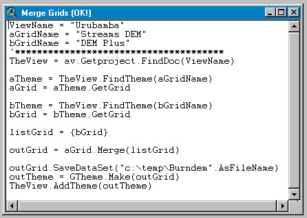
Figure 9: Merge Grids script.

Compile the script by going to Script/Compile.
Run the script by going to Script/Run. A grid called Burndem in the c:\temp directory and a theme called Burndem in the View will be created.
Fill the Burndem grid by going to Hydro/Fill.
Save the Filled Burndem grid by making it active, going to Theme/Save Data Set and writing the file name in the dialog box.

This Filled Burndem is the modified DEM.

Part II: Delineating Streams and Watersheds

As in "Part I: Setting the DEM", it is assumed a working View window, and that it contains the Filled Burndem grid-theme. The stream and watershed delineation itself is made by the Watersheds script shown in Figure 10.

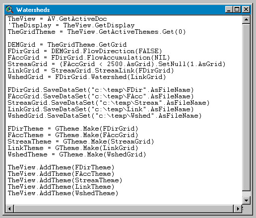
Figure 10: Watersheds script.

To run this script:

In the View window, make the Filled Burndem grid-theme active.
Open the script Watersheds, compile it if necessary by going to Script/Compile.
Run the script by going to Script/Run. Two grids, Wshed and Stream, have been created in the c:\temp directory, and their corresponding grid-themes have been added to the View.
Vectorize the Wshed grid by making it active, going to Theme/Convert to Shapefile, and writing a file name in the dialog box.

The script, as it looks in Figure 10, uses a threshold of 2500 grid cells, i.e., 2500 Km². This number, though, can be changed manually in the script according to the user needs.

The streams and watersheds, of the Urubamba River basin, delineated with this methodology are shown in Figure 11.

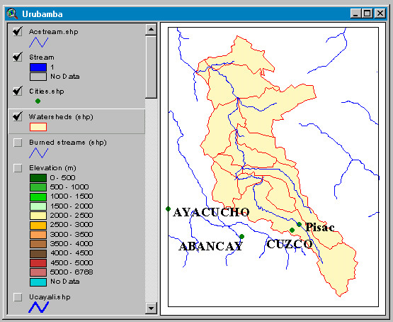
Figure 11: Delineated streams and watersheds of the Urubamba River basin.

4. Using the Hydrologic Modeling Extension

To take full advantage of the Hydrologic Modeling Extension, including the use of the W (watershed) and R (flow path) buttons and the Hydro/Watershed function, the name of the flow-direction and flow-accumulation grids should be entered in the Hydro/Properties dialog box. Once the name of these grids has been entered, the buttons and the function become active.

After making active the Filled Burndem grid-theme (regardless it is displayed or not), cliking the R button enables the flow-path function (the R button will remain depressed). Clicking on any point of the View display area will generate a flow-path line that runs from the point to its pour point or out of the analysis area. More than one point might be cliked and all the flow-paths are displayed at once. Figure 12 shows the results of applying the flow-path function in six points of the study area.

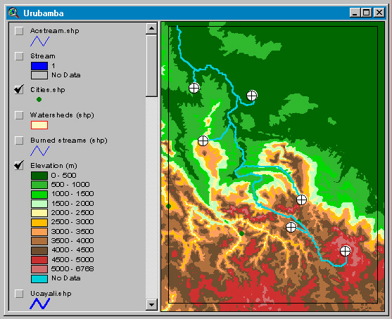
Figure 12: Using the R button to delineate flow-paths.

Clicking the W button - again with the Filled Burndem grid-theme active - enables the watershed function (the W button will remain depressed). Clicking on any point of the View display area will generate a watershed grid for the selected point. Figure 13 shows the results of applying the watershed function on the most downstream point of the Urubamba, just before its confluence with the Ene to form the Ucayali River.

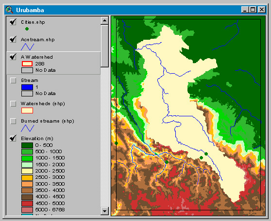
Figure 13: Using the W button to delineate watersheds.