Landslide Forecasting at the HJ Andrews
Experimental Forest Using GIS
![]()
![]()
Development of HJ Andrews Digital Watershed using ArcView GIS Tools
Creating Calibration Region Theme
![]()
![]()
This term project has been prepared to showcase one
tool that may be used to aid in educated and controlled development and related
population growth in areas of the United States susceptible to terrain
instability. The Stability Index
Approach to Terrain Stability Hazards Mapping (SINMAP) model is a program
designed to assess terrain stability conditions in the geographical information
system (GIS) framework. As presented in
this report, this tool was used to identify and map potentially unstable
regions of the HJ Andrews Experimental Forest (Figure 1.1), located
approximately 50 miles east of Eugene, Oregon.
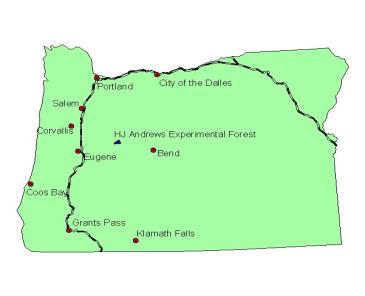
Figure 1.1 Location Map of HJ Andrews Experimental
Forest
Terrain stability has plagued the western United
States ever since adventure-seekers were tempted by promises of gold, land, and
freedom in the late 1800s. For the
people from the East and Midwest, the route west traversed rugged and difficult
land, but, inevitably, this “untamed” land began to be settled. Along with the influx of population,
however, came the haphazard use of the abundant natural resources of the
west. The necessity of transportation
yielded roads in inhospitable country; houses needed to be built, and
homesteaders turned to the forests for answers. Development continues to this day, but for the past several
decades Americans have begun to see the effects of uncontrolled growth.
Too often, this development has had adverse effects
on the natural landscape – one such example is landslides. Although they occur in every state and U.S.
territory, some areas are more vulnerable than others. The Rocky Mountains, the
Appalachian Mountains, the Pacific Coastal ranges, and parts of Alaska and
Hawaii all have areas of very weak or stressed material resting on steep slopes.
Together with the construction of homes and other structures in these areas,
heavy logging and the associated roads constructed to access harvestable
timber, and increased groundwater flows and surface water runoff due to
development, landslides have become prevalent in these areas, especially during
seasons of heavy rain and snowfall.
Mudslides have plagued California, among other states, for many years,
and Colorado had several fatal avalanches in 1999.
Determining the locations of areas potentially susceptible to these natural phenomena has become critical as the population in the west continues to strain the limits of the surrounding resources. In particular, GIS has come to light in the last decade as an effective tool to map dangerous areas throughout the United States.
The purpose of this report is to determine the
effectiveness of mapping potentially unstable areas using GIS and digital
terrain data that is readily available over the Internet. The HJ Andrews Experimental Forest was
selected because data specific to this application has been developed in the
past several years, including:
§
Digital Elevation
Models (DEMs) with a resolution fine enough to accurately represent the
terrain;
§
Groundwater recharge
data necessary to populate the model;
§
Soils data specific to
the sub-basin of interest; and
§
Maps of the locations
and types of landslides that have occurred in the sub-basin necessary to
calibrate the model.
In particular, this report will present the methodology used to define a digital representation of the terrain. The infinite slope stability model will be discussed, and the SINMAP model will be applied to the HJ Andrews site, generating a stability index for the site, as well as a map of the areas most susceptible to landslides, which will be calibrated with actual landslide data.
![]()
Development of HJ Andrews Digital
Watershed Using ArcView GIS Tools
![]()
Established in 1948 by the US Forest Service, the HJ
Andrews Experimental Forest has been the root of the HJ Andrews Long Term
Ecological Research (LTER) program - a major center for analysis of forest and
stream ecosystems in the Pacific Northwest.
Since its inception, predominantly Forest Service research has been
conducted on the management of watersheds, soils, and vegetation in the
sub-basin. LTER work has developed a backbone of long-term field experiments as
well as long-term measurement programs focused on climate, stream flow and
water quality, and vegetation succession.
During LTER3 (1990-1996) increasing emphasis was placed on developing
the concepts and tools needed to predict effects of natural disturbance, land
use, and climate change on ecosystem structure, function, and species
composition. Portions of this data have
been used for the application of the SINMAP tool to the HJ Andrews sub-basin.
With only basic terrain data, such as DEMs, GIS tools are able to provide environmentalists, natural resource planners, and developers alike with a general idea of areas most susceptible to terrain instability. ArcInfo is a powerful GIS tool used to create GIS data, while ArcView is a particular GIS tool that is capable of manipulating existing GIS data.
The first step taken to determine the potential
susceptibility of terrain to landslides in the HJ Andrews sub-basin was to
develop an accurate representation of the terrain. DEMs, readily available at
several different resolutions over the Internet (http://edcwww.cr.usgs.gov/doc/edchome/ndcdb/ndcdb.html),
are packets of data encompassing a prescribed area that provide
three-dimensional data, much like an electronic topographic map of the area. A
DEM consists of a sampled array of elevations for ground positions that are
normally at regularly spaced intervals.
DEMs can be imported into ArcView using the Spatial Analyst extension.
A DEM with a 10-meter by 10-meter cell coverage for
the HJ Andrews site was made available and imported into ArcView. The following steps were implemented to
successfully load the DEM into GIS:
1.
The file dem.asc
was imported into ArcView using the File/Import menu.
2.
The file was opened in
a text editor to ensure that the data was correct and in the proper format.
3.
The first six lines of
the file were edited in a text editor to match other ASCII DEMs. The original file read:
north: 4903755
south: 4893465
east: 572175
west: 558465
rows: 343
cols: 457
The first six lines of the file were modified to read:
ncols 457
nrows 343
xllcorner 558465
yllcorner 4893465
cellsize 10
NODATA_value -9999
This was necessary because
ArcView is designed to read this data in a particular order and for unknown
reasons, the ASCII DEM did not supply this data in the correct order.
A representation of the DEM as imported into ArcView is presented in Figure 2.1.
Figure 2.1
HJ Andrews DEM
The projection of the DEM was determined to be in
the Universal Transverse Mercator (UTM) projection, which in this case used the
North American Datum (NAD) of 1927. The
HJ Andrews site falls in Zone 10 of the UTM projection. This was determined by opening the dem.prj
text file associated with the DEM.
Determining the projection of the DEM was critical due to the fact that all of the other data layers that were to be used with the DEM had to be in the same projection, with the same cell size defined for each subsequent data layer as that of the original DEM.
Grid Clipping using CRWR-Raster
The ArcView extension CRWR-Raster was used to clip
the DEM grid to fall entirely within the limits of the Boundary
theme. With the DEM grid active, the
steps followed included:
1.
Select
CRWR-Raster/Clip Grid by Polygon
2.
Select Yes to clip
active theme by polygon to be chosen
3.
Select Boundary as
Clipping Theme
A new DEM grid was generated that had all the elevation values completely within the Boundary theme.
Landslides
Landslide data specific to the HJ Andrews site was a
critical piece of information for this site, eventually used to calibrate the
SINMAP model. The landslide data was
downloaded in ArcInfo format (the file had a .e00 extension) and was
imported into ArcView using the Import 71 feature.
The landslide data was added as a point coverage
theme, with each point having attributes of area, perimeter, slide id, slide #,
id, northing, and easting.
The projection for the landslide data was also
determined to be in the UTM – NAD 27 Zone 10 projection, so no additional
projection was necessary.
In order to successfully calibrate the SINMAP model,
a field called Type had to be defined for each point. Initially, there was no Type field
associated with each landslide. This
data was gathered from personnel at the HJ Andrews site and was added manually
to the attribute table of the point coverage.
With the Attributes to Slides theme active, the Type field
was added using the following steps:
1.
Select Table/Start
Editing
2.
Select Edit/Add Field
3.
At the Name
prompt, input Type
4.
Manually enter the
landslide type for each point
5.
Select Table/Save
Edits
6.
Select Table/Stop
Editing
The landslide type was differentiated between those
that started as a result of road construction (2) and those unrelated to road
construction (1). This allowed the
calibration of the SINMAP model with only the naturally occurring landslides
and gave a more true representation of the areas of the sub-basin susceptible
to landslides due to terrain and moisture conditions in the soil.
Figure 2.2
Type Field in Landslide Attribute Table
Soils
Soils data for the HJ Andrews sub-basin was also
downloaded. This included soils data
specific to the HJ Andrews site available on the project web site in addition
to State Soil Geographic (STASGO) database data downloaded from the USGS (http://www.ftw.nrcs.usda.gov/statsgo2_ftp.html)
The soils data specific to the HJ Andrews sub-basin
was downloaded from the project web site in ArcInfo format and imported into
ArcView using the Import 71 feature.
The attributes associated with this data included:
§
Area
§
Perimeter
§
Soil Survey #
§
Soil Survey ID
§
Soil Unit
§
Unit Name
§
Description
§
Slope Class
§
Depth Class
§
Land Type
§
Map Symbol
§
Map Unit
This site-specific data can be related to the STATSGO soils data (presented below) via the Map Unit and Soil Unit fields.
This data set is a digital general soil association
map developed by the National Cooperative Soil Survey and consists of a broad
based inventory of soils and non-soil areas that occur in a repeatable pattern
on the landscape. The STATSGO soil maps are compiled by generalizing more
detailed soil survey maps. The soil map units are linked to attributes in the
Map Unit Interpretations Record relational database, which gives the
proportional extent of the component soils and their properties in each map
unit.
STATGSO was designed primarily for regional,
multi-county, river basin, state, and multi-state resource planning and, as
such, the large size of the polygons makes it suitable only for large areas.
Another database, called SSURGO (still under development by the USDA), details
soil polygons on the component level as opposed to the map unit level and would
be more suitable to small coverages like the HJ Andrews sub-basin.
The STATSGO soils coverage for the State of Oregon
was downloaded as a polygon shape file and was imported as a theme into
ArcView. The projection of the data was
originally in the Albers Equal Area projection, so it had to be projected to
the UTM-NAD 27 Zone 10 projection to match the other themes in ArcView. The CRWR-Vector extension was used to project
this theme. With the STATSGO
theme active, the steps followed included:
1.
Select Output Units
of meters
2.
Select UTM-NAD 27
from the Category menu
3.
Select Zone 10
from the Type menu
A new polygon coverage of the STATSGO soils was created in the proper projection, and the polygon theme was then clipped using the ArcView Geoprocessing Wizard extension described below.
Additional data
downloaded from the HJ Andrews web site included:
§
The boundary of the HJ
Andrews watershed, added as a polygon theme;
§
Detailed road maps of
the sub-basin, added as a polygon theme;
§
50 ft. contours of the
sub-basin, added as a polygon theme; and
§
Stream gauge
locations, added as a point theme.
As with the rest of the data downloaded from the HJ Andrews web site, the data had to be imported into ArcView using the Import 71 feature.
Clipped Grids (Geoprocessing Wizard)
The ArcView extension Geoprocessing Wizard was used
to clip the Roads and Contours polygons to match the boundary of
the HJ Andrews sub-basin. With the Boundary
Theme active, the steps included:
1. Select View/Geoprocessing Wizard
2. Select Clip on theme based on another
3. Select Boundary as Input Theme to Clip by
4. Select Roads or Contours as Polygon Overlay Theme
A new polygon theme was then generated that fell entirely within the Boundary theme. A three-dimensional representation of the entire HJ Andrews watershed with select themes activated is presented in Figure 2.3.
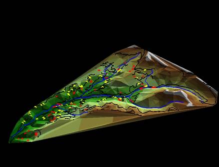
Figure 2.3
HJ Andrews Watershed with Select Themes Activated
This view was created with the 3-D Analyst ArcView
extension. The 3-D Analyst used the HJ
Andrews DEM to create a triangular irregular network (TIN) to represent the
topography. A clipped RF3 file from the
EPA Basins web site was overlayed on the TIN, along with the roads theme, to provide
the user with reference points. The red
dots represent landslides that occurred naturally, while the yellow dots
represent landslides that occurred in close proximity to roads.
![]()
![]()
SINMAP is a grid-based ArcView extension developed
at Utah State University with the support of Forest Renewal British Columbia,
in collaboration with Canadian Forest Products Ltd., Vancouver, B.C. This program implements the computation and
mapping of a slope stability index based upon geographic information, primarily
digital elevation data. As applicable
to the HJ Andrews experimental forest, SINMAP was the logical tool for the
prediction of the areas most susceptible to landslides because it could be
populated with site-specific data (gathered over the last several years) to
quickly identify regions where more detailed terrain stability assessments may
be warranted.
There are many approaches to assessing slope stability
and landslide hazards. Field inspection
has been the most widely used approach historically, but this is an arduous
process that is time-consuming and expensive.
The projection of future instability patterns from documented landslide
types and locations has also been used extensively, but this method may not
account for site-specific environmental conditions in all cases. The purpose of the SINMAP software is to
provide an objective terrain stability mapping tool that can compliment the
subjective terrain stability mapping methods currently being practiced in the
field.
SINMAP relies heavily on the coupling of steady
state topographic hydrologic models with the infinite plane slope stability
model, and has its theoretical basis in the infinite plane slope stability
model with wetness (pore pressures) obtained from a topographically based
steady state model of hydrology. SINMAP
uses site-specific data, combined with past landslide history, to create a
probabilistic model of the terrain most susceptible to instability.
It is important for the reader to note that a large part of the text of this section was taken directly from the SINMAP User’s Guide, 1998. For a more in-depth discussion of the theory of the SINMAP model, the reader is referred to this document.
The SINMAP methodology is based upon the infinite
slope stability model (e.g., Hammond et al., 1992; Montgomery and Dietrich,
1994) that balances the destabilizing components of gravity and the restoring
components of friction and cohesion on a failure plane parallel to the ground
surface with edge effects neglected.
Soil moisture (specifically, pore pressure) is also taken into
consideration in this model because it reduces the effective normal stress on
the failure plane. SINMAP populates the
topographic variables of the slope stability model by automatically extracting
elevation data from the DEM, calculating the specific catchment area (sub-basin)
of each cell, and quantifying the corresponding material properties in the
sub-basin on a cell-by-cell basis, such as soil strength and the effects of
climatological factors. The primary
output of the SINMAP model is a stability index used to classify the terrain
stability in each grid cell within the study area.
The following input parameters are recognized to
vary in each sub-basin and are specified in SINMAP by the user as upper and
lower boundaries on the ranges these values may take:
§
T/R
§
Cohesion
§
Angle of Internal
Friction
§
Lower Wetness Line
Percentage
The first parameter listed above is the ratio of
transmissivity of the soil (m2/hr) to the effective steady-state
lateral recharge rate of the groundwater in the sub-basin (m/hr), with a
default range of 2000 to 3000 (m).
Transmissivity data is collected in the field and is specific to each
soil type in the sub-basin of interest.
As such, it is difficult to quantitatively estimate specific values for
both transmissivity and recharge and, thus, SINMAP uses a range of values to
model the uncertainty of these values.
The second parameter is the cohesive properties of
the soils of the sub-basin, with a default range of 0 to 0.25
(dimensionless). This data is also
collected in the field and, for the same reasons described above, is input as a
range of values.
The third parameter is the angle of internal friction (F), with a default range of 30 to 45 degrees. Although the actual angle of internal friction for specific soils can only be determined in the field, F can be determined in general terms from Table 3.1, extracted from the Standard Handbook of Civil Engineering (McGraw-Hill, 1995).
Table 3.1
Angles of Internal Friction and Unit Weights of Soils
|
Type of Soil |
Density or Consistency |
Angle
of Internal Friction, Phi, degrees |
Unit
Weight (lb/ft3) |
|
Coarse
Sand or Sand
and Gravel |
Compact Loose |
40 35 |
140 90 |
|
Medium
Sand |
Compact Loose |
40 30 |
130 90 |
|
Fine
Silty Sand or Sandy
Silt |
Compact Loose |
30 25 |
130 85 |
|
Uniform
Silt |
Compact Loose |
30 25 |
135 85 |
|
Clay-Silt |
Soft to
Medium |
20 |
90-120 |
|
Silty
Clay |
Soft to
Medium |
15 |
90-120 |
|
Clay |
Soft to
Medium |
0-10 |
90-120 |
The last parameter is the SA plot lower wetness line
percentage. This dimensionless value
represents the boundary wetness between the low moisture and partially wet
zones on the saturation map. It is also
the wetness of the lowest line on the SA plot.
Table 3.2 provides an example of the stability classes that are defined in terms of the Stability Index (SI) for this model. The SI is the factor of safety that gives a measure of the magnitude of destabilizing factors required for terrain instability and is defined as the probability that a location is stable assuming uniform distributions of the parameters over the uncertainty ranges specified above. The SI generally ranges between 0 (most unstable) and 1.0 (least unstable). However, where the most conservative set of parameters still result in stability, the stability index is defined as the factor of safety at this location under the most conservative set of parameters and may yield a value greater than 1.0.
Table 3.2
Stability Class Definitions
|
Condition |
Class |
Predicted
State |
Parameter
Range |
Possible
Influence of Factor Not Modeled |
|
SI >
1.5 |
1 |
Stable
slope Zone |
Range
cannot model instability |
Significant
destabilizing factors required for instability |
|
1.5
> SI > 1.25 |
2 |
Moderately
stable slope zone |
Range
cannot model instability |
Moderate
destabilizing factors required for instability |
|
1.25
> SI > 1.0 |
3 |
Quasi-stable
slope zone |
Range
cannot model instability |
Minor
destabilizing factors could lead to instability |
|
1.0
> SI > 0.5 |
4 |
Lower
threshold slope zone |
Pessimistic
half of range required for instability |
Destabilizing
factors are not required for instability |
|
0.5
> SI > 0.0 |
5 |
Upper
threshold slope zone |
Optimistic
half of range required for instability |
Stabilizing
factors may be responsible for stability |
|
0.0
> SI |
6 |
Defended
slope zone |
Range
cannot model instability |
Stabilizing
factors are required for stability |
The selection of breakpoints (1.5, 1.25, 1.0, 0.5
and 0.0) in Table 3.2 is subjective, requiring user judgment and interpretation
in terms of the class definitions. The
terms ‘stable’, ‘moderately stable, and ‘quasi-stable’ are used to classify
regions that, according to the model, should not fail with the most
conservative parameters in the parameter ranges specified. The terms ‘lower threshold’ and ‘upper
threshold’ are used to characterize regions where, according to the parameter
uncertainty ranges, the probability of instability is less than or greater than
50%, respectively. The term ‘defended
slope’ is used to characterize regions where, according to the model, the slope
should be unstable for any parameters within the parameter ranges
specified. In general, if the SI is
greater than 1.0, there is a probability that the terrain is unstable given the
most conservative parameters specified in the user-defined ranges.
The general infinite slope stability model factor of safety (ratio of stabilizing to destabilizing forces) is given by (simplified for wet and dry density the same, from Hammond et al., 1992):
![]()
where:
![]()
Figure 3.1 presents a graphical representation of
the parameters described above.
Figure 3.1
Infinite Slope Stability Model Schematic
The SINMAP model makes a few simplifications to the
above model. It interprets the soil
thickness as specified perpendicular to the slope, rather than soil depth
measured vertically. Soil thickness, h
(m) and depth are related as follows:
![]()
With this change, the
factor of safety reduces to:
![]()
where:
This
is the dimensionless form of the infinite slope stability model used in the
SINMAP model. This
equation is convenient to use because cohesion (due to soil and root
properties) is combined with the soil density and thickness into a
dimensionless cohesion factor C. This
may be thought of as the ratio of the cohesive strength relative to the weight
of the soil, or the relative contribution to slope stability of the cohesive
forces. This concept is illustrated in
Figure 3.2.
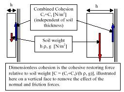
Figure 3.2
Illustration of Dimensionless Cohesion Factor Concept
The second term in the new factor of safety equation
quantifies the contribution to stability due to the internal friction of the
soil (as quantified by the friction angle F, or friction coefficient tan
F). This is reduced as wetness
increases due to increasing pore pressures and consequent reductions in the
normal force carried by the soil matrix.
The sensitivity to this effect is controlled by the density ratio, r.
However, relative wetness, as defined above, can be further explained as detailed below. Field observations have noted that the higher soil moisture or areas of surface saturation tend to occur in convergent hollow areas in the topography. Similarly, it has also been reported that landslides most commonly originate in areas of topographic convergence. For these reasons, the concept of specific catchment area ‘a’ can be used to determine the relative wetness of the soil at any location within a sub-basin (see SINMAP User’s Manual, 1998 for further explanation), and is defined as:
![]()
The relative wetness has an upper bound of 1, with
any excess assumed to form overland flow.
This relative wetness defines the relative depth of the perched aquifer
within the soil layer of interest. The
ratio R/T, which has units of m-1, quantifies the relative wetness
in terms of assumed steady state recharge relative to the soil’s capacity for
lateral drainage of water. It is
important to note that the quantity R is not a long-term average of recharge,
but rather it is the effective recharge for a critical period of wet weather
likely to trigger landslides. The ratio
R/T, which SINMAP treats as a single parameter, therefore combines both climate
and hydrological factors.
Therefore, to define the stability index, the wetness index from above is incorporated into the dimensionless SINMAP factor of safety equation, which becomes:
The variables a and T are derived from the
topography, with C, tan F, r, and R/T parameters specified by the user. SINMAP treats the density ratio as
essentially constant (with a value of 0.5), but allows uncertainty in the other
three quantities through the specification of lower and upper bounds.
For areas where the minimum factor of safety is
greater than 1, there is a probability of failure. This is a spatial probability due to the uncertainty in C, tan F,
and T. This probability does have a
temporal element in that R characterizes a wetness that may vary with time.
Practically, the SINMAP model works by computing slope and wetness at each grid point, assuming other parameters are constant (or have constant probability distributions) over large areas. With the form of the new factor of safety equation, this amounts to implicitly assuming that the soil thickness (perpendicular to the slope) is constant.
Grid DEMs were selected to represent topography in
SINMAP primarily due to their simplicity and compatibility with ArcView Spatial
Analyst grid routines, as well as the availability of data and prior experience
with their use. The grid processing
routines consist of four main steps:
§
Pit filling
corrections;
§
Computation of slopes
and flow directions;
§
Computation of
specific catchment area; and
§
Computation of the
SINMAP stability index.
Pits in DEMs are defined as grid elements or sets of
grid elements surrounded by higher terrain that, in terms of the DEM, do not
drain to adjacent cells. These are rare
in natural topography and are generally assumed to be due to errors in the
generation of the DEM. They are
eliminated in SINMAP by using the “flooding” approach, essentially raining the
elevation of each pit grid cell within the DEM to the elevation of the lowest
adjacent grid cell. This approach is
the same that is used in the CRWR-PrePro ArcView extension studies in this
class.
Slopes and flow directions have traditionally been accomplished using the eight-direction pour point model (CRWR-PrePro uses the eight-direction pour point model). In this method, water can flow from one cell to only one of the eight surrounding cells in the grid (to the lowest of the eight surrounding grid cells). SINMAP uses the D-infinity method developed by Tarboton (1997). In this method, the flow direction angle, measured counter-clockwise from east, is represented as a continuous quantity between 0 and 2? radians. The specific angle is determined as the direction of the steepest downward slope on the eight triangular facets formed in a 3 x 3 grid cell window centered on the grid cell of interest as illustrated in Figure 3.3.
Figure 3.3
Flow Direction Defined as the Steepest Downward Slope
on Planar Triangular Facets on a Block-centered Grid
A block-centered representation is used with each
elevation value taken to represent the elevation of the center of the
corresponding grid cell. Eight planar
triangular facets are formed between each grid cell and its eight
neighbors. Each of these has a
downslope vector which, when drawn outwards from the center, may be at an angle
that lies within or outside the 45-degree angle range of the facet at the
center point. If the slope vector angle
is within the facet angle, it represents the steepest flow direction on that facet. If the slope vector angle is outside a
facet, the steepest flow direction associated with that facet is taken along
the steepest edge. The slope and flow
direction associated with the grid cell is taken as the magnitude and direction
of the steepest downslope vector from all eight facets. This is implemented using equations give by Tarboton
(1997).
In the case where no slope vectors are positive
(i.e., flat areas), the cell drains away from high ground towards low
ground. The procedure to determine flow
direction will not be discussed here because these flat areas can be considered
unconditionally stable.
Specific catchment areas are calculated using a
recursive procedure that is an extension of the very efficient recursive
algorithm for single directions (Mark, 1998).
The upslope area of each grid cell is taken as its own area (one) plus
the area from upslope neighbors that have some fraction draining to it. The flow from each cell all drains to one
neighbor if the angle falls along a cardinal or diagonal direction, or is on
the angle falling between the direct angle to two adjacent neighbors. In the latter case, the flow is proportioned
between these two neighbor cells according to how close the flow direction
angle is the to direct angle to those cells.
Specific catchment area, a, is then upslope area per unit contour
length, taken in this case as the number of cells times grid cell size. This assumes that grid cell size is the
effective contour length, and does not distinguish any difference in contour
length dependent on the flow direction.
Computation of SINMAP stability index is simply a grid cell by grid cell evaluation of the equations presented in Section 3.1.1.
The SINMAP model utilizes a library of computer
routines than can be called to perform computational tasks including
calculating stability index and degree of saturation. Additionally, library routines are also available to perform many
basic tasks of manipulating DEM grid data including pit filling, slope
calculation, flow direction calculation, and drainage area calculation. SINMAP utilizes ArcView GIS software to
carry out the tasks listed above.
ArcView version 3.0 (or later) is required to run the SINMAP modeling
extension, as is the Spatial Analyst extension, which is an add-on to the
standard ArcView GIS software package.
The software must be run on Windows 95 or Windows NT operating systems.
The SINMAP extension is a customized extension to
ArcView that provides links between ArcView and the library or routines in the
SINMAP dynamic link library. The Sinmap.avx
file must be copied to the ESRI/av_gis30/ArcView/Ext32 folder prior to
using ArcView. Similarly, the Sinmap.dll
file must be copied to the ESRI/av_gis30/ArcView/Bin32 folder prior to
starting ArcView.
The final output of most SINMAP studies will be maps
that can be used to define areas of potential terrain instability. Most tasks are conducted in SINMAP’s DEM
map window. Upon completion of
the SINMAP routines, nine GIS themes will be created in the DEM map
window.
In addition to the geographic display of study data
in the DEM map window, SINMAP also generates a slope-area chart
of study area data to aid in data interpretation and parameter
calibration. The SA Plot window
plots four types of information:
§
Normal cell data:
Specific catchment area versus slope is plotted for a sampling of grid cell
points across the study area that does not have landslides.
§
Landslide cell
data: Landslides are plotted based upon
the slope and specific catchment area values of the cell in which each
landslide point lies.
§
Stability Index region
lines: These 5 lines provide boundaries
for regions within slope-specific catchment area that have similar potential
for landslides.
§
Saturation region
lines: These 3 lines provide boundaries
for regions within slope-specific catchment areas that have similar wetness
potential.
The goal of model calibration is to adjust the stability index region lines and the saturation region lines such that the majority of the known landslides in the area fall in those areas most susceptible to terrain instability (i.e., areas where the stability index is greater than 1.0).
Implementation
The implementation of the SINMAP model was
contingent on an accurate representation of the terrain, landslide locations
and types, and soil parameters within the HJ Andrews watershed. The development of this data was presented
in Section 2.0. The following sub-sections
describe the actual implementation of the SINMAP model at the HJ Andrews
watershed.
The first step in determining a terrain instability
map for the HJ Andrews watershed was defining the model parameters. The Set Defaults menu was selected
and the following values were available for editing:
§
Gravity constant: 9.81
m/s2
§
Soil Density: 2000
kg/m3
§
Water Density: 1000
kg/m3
§
Number of points in SA
Plot: 2000
These values were
acceptable and were not edited.
The Set Calibration Parameters menu was then
selected and the following four parameters were available for editing:
§
T/R ratio: 2000-3000 m
§
Dimensionless
cohesion: 0.0-0.25
§
Angle of internal
friction: 30-45 degrees
§
Lower wetness line
percentage: 10%
Discussions with HJ Andrews personnel did not yield
site-specific data for transmissivity or lateral recharge rate, so the default
range of 2000 – 3000 meters was used.
HJ Andrews personnel did not have data on the cohesive properties of the
soil either, so the default values were again used.
Data was available for the angle of internal
friction, so several calibration region themes were developed based on the
different soil types in the region.
This process is described in Section 3.2.3 below.
The lower wetness line percentage value of 10% was used in this study.
The HJ Andrews DEM was selected for SINMAP analysis
using the Select DEM Grid for Analysis command from the SINMAP
menu. The clipped grid (representing
the boundary of the HJ Andrews sub-basin) was not used as the DEM for analysis
due to the need to have a buffer around the sub-basin to minimize the edge
effects during SINMAP processing.
Instead, the entire projected DEM was used.
Creating Calibration Region Themes
Unfortunately, the site-specific soils data supplied
by HJ Andrews personnel did not have the necessary attributes to impact the
SINMAP modeling procedure. Instead,
STATSGO soils data was used to create four calibration region themes.
The calibration region themes were developed to
further narrow the scope of uncertainty in the four calibration parameters
listed in Section 3.2.1. STATSGO data
was clipped to match the boundary of the HJ Andrews watershed, and the map unit
ID was used to join the Clipped STATSGO attribute table to the layer.dbf
table, using the following commands:
1.
Under the Table
menu in the Project window, a new table was opened (layer.dbf).
2.
The Clipped STATSGO
attribute table was selected.
3.
The Muid field
was highlighted.
4.
The layer.dbf
table was then selected.
5.
The Muid field
was highlighted in this table.
6.
Under the Table
menu, the Join command was used to join the fields of the layer.dbf
table to the Clipped STATSGO attribute table.
The layer.dbf table contained a field named Unified, which listed the Unified Soil Classification for the soils in each respective map unit (Figure 3.4). By comparing the Unified Soil Classification of each map unit within the HJ Andrews watershed to Table 3.1, an educated estimate could be made of the range of the angle of internal friction of the soils in each map unit.
Figure 3.4
Clipped STATSGO Attribute Table with Layer.dbf Attributes
Attached
The calibration region themes were then selected
using the following commands:
1.
Under the SINMAP menu,
the Create Multi-Region Calibration Theme command was selected.
2.
The Clipped STATSGO
polygon coverage (that included the four calibration region themes) was
selected.
At this point, four calibration region themes were defined, each based on the unique range of the angle of internal friction of the soils in that area (Figure 3.5).
Figure 3.5
Four Calibration Region Themes
The fourth calibration region, found in the extreme southwestern
corner of the watershed, was extremely small and did not factor into the
calibration of the model since no landslides occurred within the limits of the
region. Similarly, HJ Andrews personnel
have not documented any known landslides in the area represented in purple in
Figure 3.5, so this region was not included in the calibration of the model
either.
The landslide point theme was added to the DEM: Dem
view window by selecting Select Landslide Point Theme from the SINMAP
menu.
SINMAP was then used to develop the following grids
based on the data input above:
§
Pit-Filled DEM
§
Flow Direction Grid
§
Slope Grid
§
Contributing Area Grid
The flow direction grid is presented in Figure 3.6, and the Contributing Area Grid is presented in Figure 3.7.
Figure 3.6 Flow Direction Grid Figure 3.7 Contributing Area Grid
The grids developed above were derived solely from
the DEM grid and required no other parameters for their construction. As such, these grids form the basis of the
stability analysis and are not changed even if the calibration parameters are
adjusted.
All data necessary to develop the saturation grid
and the stability index grid was now available. Under the Stability Analysis menu of the SINMAP
menu, Compute all steps was selected.
SINMAP then calculated the two grids for the Calibration Region themes
defined above. The Stability Index Grid
is presented in Figure 3.8, and the initial SA Plot is presented in Figure 3.9.
Figure 3.8 Initial Stability Index Grid Figure 3.9 Initial SA Plot Prior to Calibration
Prior to Calibration
At this point, calibration of the results was
desired based on the attributes of the landslide point coverage and the
calibration region themes defined previously.
Although the calibration parameters for each them can be adjusted in the
DEM view window, calibration of the model was more effectively conducted in the
SA Plot window.
To calibrate the model effectively, each calibration
region theme was modified individually.
With the angle of internal friction specified for each theme, only the
T/R ratio and dimensionless cohesion parameters needed to be adjusted. As stated previously, the goal of
calibration is to adjust the stability index and saturation region lines on the
SA Plot to maximize the number of natural landslides occurring the regions
where the SI is greater than 1.0 (specifically, in the ‘lower-threshold slope
zone’, the ‘upper threshold slope zone’, and the ‘defended slope zone’).
A representation of the calibrated Map Unit OR64 landslides is depicted in Figure 3.10.
Figure 3.10
Calibrated Map Unit OR64 SA Plot
Upon completion of this step, viewing the statistics
of each calibration region theme can check calibration of the model. It is important to maximize the landslide
density in the potentially unstable zones listed above, and the statistics menu
allows the user to determine the applicable landslide densities. To view the statistical summary window, the
user right-clicks on the mouse in the SA Plot window and selects Statistics. This window also provides information for
each calibration region theme on:
§
The area in square
kilometers;
§
The percentage of area
in each stability zone;
§
The number of
landslides;
§
The percentage of
landslides in each stability zone; and
§
The landslide density
in # per square kilometer.
Figure 3.11 presents the statistical summary window for the calibrated map unit OR64 calibration region theme.
Figure 3.11
Statistical Summary of the Map Unit OR64 Calibration Region Theme
![]()
![]()
The results of the SINMAP terrain stability model
for the HJ Andrews site is presented in this section. Overall, the model performed well, but additional site-specific
data would be beneficial in populating the calibration parameters.
Figure 4.1 presents the final output of the SINMAP
model for the HJ Andrews watershed. As
can be seen, the locations of landslides match the modeled terrain instability
in most cases.
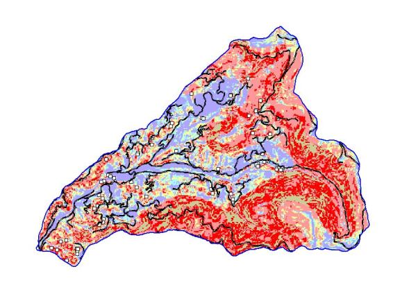
Figure 4.1
Final Output of SINMAP Model for HJ Andrews Watershed
The white squares in Figure 4.1 present the
locations of known landslides in the HJ Andrews watershed. The color scheme for the figure is as
follows:
§
Blue: Stable (SI >
1.5)
§
Aqua: Moderately
Stable (1.5 > SI > 1.25)
§
Tan: Quasi-stable (1.25 > SI > 1.0)
§
Pink: Lower Threshold
(1.0 > SI > 0.5)
§
Red: Upper Threshold
(0.5 > SI > 0.0)
§
Brown: Defended (0.0
> SI)
The areas that are the most stable can be found in
the flattest regions of the watershed, namely along the creek bottom. Limited landsliding has occurred in these
areas, but this can be attributable to shear stress on the banks in the form of
erosion. The areas of greatest
instability also match well with the steepest terrain. Overall, the model does well, placing 90.1%
of the landslides in the OR64 calibration region theme in the zones with a SI
less than 1.0, and placing 46.9% of the landslides on the OR78 calibration
region theme in the same zones. The
outlying data points are most often landslides located near roads, lending
further credence to the model’s output.
Comparison
to USGS Map
The United States Geological Survey has produced a large-scale map of potentially unstable terrain in the United States that may be susceptible to landslides (Figure 4.2).
Figure 4.2
USGS Landslide Overview Map of the United States
The USGS methodology is to differentiate those areas
known to have experienced landslides from areas that are merely susceptible to
terrain instability and may not have experienced a landslide to date. The map units were classified into three
incidence categories, according to the percentage of the area involved in
landslide processes:
|
Area involved in
Landsliding |
Incidence |
|
Greater
than 15% |
High |
|
From
1.5% to 15% |
Medium |
|
Less
than 1.5% |
Low |
This rationale is similar to the rationale for
calibration of the SINMAP model. The
statistical summary window that can be generated from the SA Plot provides the
percentage of the watershed of interest that can be considered susceptible to
landslides, as well as the percentage of the slides that have occurred in each
area.
A comparison of the SINMAP model output to the USGS
map is made here to show the increased resolution available in the SINMAP
model.
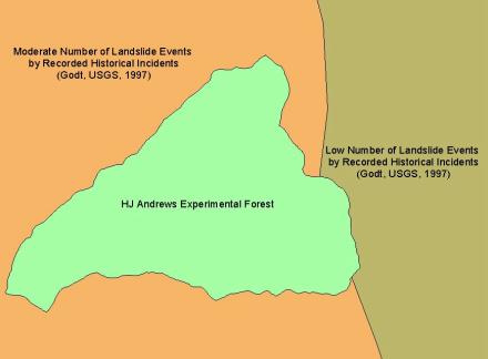
Figure 4.3
USGS Landslide Overview Map Compared to the HJ Andrews Watershed
It is evident from Figure 4.3 that the SINMAP output
presented in Figure 4.1 is a much more detailed representation of the local
terrain of the HJ Andrews watershed.
Although undertaking the mapping of the entire United States with a
model such as SINMAP is currently limited by computer processing speeds and
memory, perhaps in the future a more detailed analysis of the terrain of the
United States will be possible.
![]()
![]()
The report has shown that the use of GIS tools to
model terrain instability can be effective in predicting potentially unstable
terrain. As development continues to
encroach upon the natural areas of the United States, models such as SINMAP
will become invaluable in educating developers, land owners, logging companies,
government entities, and environmentalists alike as to the susceptibility of
the terrain to landslides and other similar phenomena.
The rationale for developing digital terrain data
was presented and provided an accurate representation of actual field
conditions. The data used is available to the public over the World Wide Web,
along with the SINMAP model, so this procedure can be used without much
difficulty.
As more specific soils data becomes available (SSURGO), a more complete understanding of the effects of groundwater and soil-pore moisture on the terrain instability will be possible. In particular, existing STATSGO (and in the future, SSURGO) soils data contains attributes that are directly applicable to use in this model. The following soil data elements may be of use in the future in determining terrain instability using SINMAP:
§
Available Water
Capacity
§
Bulk Density
§
Clay
§
Soil Drainage Class
§
Hydrologic Group
§
Layer Depth
§
Liquid Limit
§
Percent Passing
Various Sieve Sizes
§
Depth to Cemented Pan
§
Particle Size
§
Permeability Rate
§
Plasticity Index
§
Ponding Depth
§
Depth to Bedrock
§
Shrink-Swell Potential
§
Soil Slope
§
Total Subsidence
§
Surface Soil Texture
§
Unified Soil
Classification (used in this analysis)
§
Water Table Depth
§
Seasonal Water Table
Existence and Depth
The modification of the SINMAP model to make use of the above parameters would be a tremendous step in ensuring that integration of natural areas with development occurs in the best possible manner for all involved.
![]()
![]()
97-289 - Digital Compilation of “Landslide Overview
Map of the Conterminous United States” By Dorothy H. Radbruch-Hall, roger B.
Colton, William e. Davies, Ivo Lucchitta, Betty A. Skipp, and David J. Varnes,
1982; USGS Open-File Report 97-289 by Godt, Jonathan W., 1997.
Beven, K., R. Lamb, P. Quinn, R. Romanowicz and J.
Freer, (1995), "TOPMODEL," Chapter 18 in Computer Models of Watershed
Hydrology, Edited by V. P. Singh, Water Resources Publications, Highlands
Ranch, Colorado, p.627-668.
Maidment, David R. Handbook of Hydrology. New York:
McGraw-Hill, 1992.
Merrick, Frederick S., M. K. Loftin, and J. T.
Ricketts. Standard Handbook for Civil
Engineers, Fourth Edition. New York:
McGraw-Hill, 1996.
Pack, R. T., D. G. Tarboton and C. N. Goodwin,
(1998), “SINMAP User’s Manual”, 1998 (available online at http://www.engineering.usu.edu/cee/faculty/dtarb/sinmap.pdf).
Pack, R. T., D. G. Tarboton and C. N. Goodwin,
(1998), "The SINMAP Approach to Terrain Stability Mapping," 8th
Congress of the International Association of Engineering Geology, Vancouver,
British Columbia, Canada 21-25 September 1998. (available online at http://www.engineering.usu.edu/dtarb)
Tarboton, D. G., (1997), "A New Method for the
Determination of Flow Directions and Contributing Areas in Grid Digital
Elevation Models," Water Resources Research, 33(2): 309-319. (available online
at http://www.engineering.usu.edu/dtarb)
Veismann, Warren Jr., G.L. Lewis, and J.W.
Knapp. Introduction to Hydrology, Third Edition. New York:
HarperCollins, 1989.
HJ Andrews Experiment Forest – Long Term Ecological
Research Web site: http://sequoia.fsl.orst.edu/lter/
USDA - Natural Resources Conservation Service Web
site: http://www.ftw.nrcs.usda.gov
US EPA Web site: http://www.epa.gov
USGS National Landslide
Information Center:
http://landslides.usgs.gov/html_files/nlicsun.html
USGS Web site: http://www.usgs.gov